This page has been permanently moved. Please
CLICK HERE to be redirected.
Thanks, Craig.
Have you ever wondered why tuning Oracle improves performance? There are of course obvious answers, but then there are the deeper answers. More profound answers. It's like answering the question, "Why is the sky blue?" Sure you can say, it because the sun's light rays are scattered when they hit the Earth's atmosphere. But then why does scattering the light rays turn the sky blue? And it goes on and on. It can be just like that with Oracle performance.Last month I blogged about CBC latches, CPU consumption, and wait time. In that posting I demonstrated that by adding cache buffer chain (CBC) latches to a CBC latch constrained system the CPU consumption per logical IO decreased.
In this posting I want to demonstrate how a change in CPU consumed per logical IO causes a corresponding change in the time it takes to process a logical IO...just as Operations Research queuing theory states.
Note: When I write, "tuning Oracle" I am referring to altering instance parameters that do not influence the optimizer to change a SQL statement's execution path. For this posting, I'm typically referring to instance parameters that alter the number of cache buffer chains and latches.
For many of you, this posting will be immensely satisfying because we will have quantified and modeled the Oracle system, taken a tuning solution and quantitatively observed and understood why it altered the system, and then we observed the result closely matched our quantitative model. If this still seems overly theoretical, in the next blog entry you will see how we can use this understanding to anticipate the impact on a SQL statement's elapsed time!
In my previous CBC latches, CPU consumption, and wait time posting I defined and used a few terms that must be understood before this blog posting will make any sense. The terms are unit of work, service time, queue time, response time, arrival rate, and elapsed time. Response time is the time to complete a single unit of work and elapsed time is the time to process multiple units of work. If this is somewhat confusing, please refer to that previous blog entry.
The Experimental Setup
To meet my objectives I created an experiment that is easily repeatable. I created a massive CPU bottleneck by having a number of Oracle sessions run SQL where all their blocks reside in the buffer cache, that is SQL is logical IO (v$sysstat: session logical reads) dependent. I gathered 30 ten minute samples with the CBC latches set to 256 and then to 32768. During these ten minute collection periods, I sampled the elapsed time of a specific LIO dependent SQL statement. With 256 CBC latches, around 23 elapsed times where collected. With 32768 CBC latches, around 71 elapsed times where collected. The difference in the number of elapsed time samples was the result of the SQL completing sooner when there was 32768 CBC latches.
If you look closely at my data collection script, you can easily see how I captured, stored, and retrieved the performance data. You can download the data collection script here. The SQL elapsed times where gathered using the OraPub SQL Elapsed Time Sampler.
You can download the raw data text files (256 latches, 32768 latches) and the Mathematica analysis notebook (PDF, notebook).
Concepts/Terms Quickly ReviewedIf you look closely at my data collection script, you can easily see how I captured, stored, and retrieved the performance data. You can download the data collection script here. The SQL elapsed times where gathered using the OraPub SQL Elapsed Time Sampler.
You can download the raw data text files (256 latches, 32768 latches) and the Mathematica analysis notebook (PDF, notebook).
Unit of Work Time
Current Oracle performance analysis focuses much on the time involved (CPU plus non-idle wait time) related to SQL statement completion, process completion, or an Oracle instance over an specified interval (think: Statspack/AWR). That's great and is a fantastic analysis leap forward from ratio analysis and wait event analysis because it better reflects what a user is experiencing and it includes both wait time and CPU consumption. But to unite Oracle time based analysis with Operations Research queuing theory, we need the time related to a specific piece (or unit) of work. When we do this, we gain the advantages of our Oracle analysis plus all the years of proven Operations Research! Yeah... it's a big deal.
There are many ways to describe the work being processed in an Oracle system. When we say, "The LIO workload is unusually high today" we are relating performance to the LIO workload. Or how about, "Parsing is hammering performance!" or "Disk reads are intense and really slow today and it's affecting some very key SQL statements." Each of these statements is speaking and relating system performance to a type of work; namely logical IO (session logical reads), parsing (parse count (hard)), and disk reads (physical reads).
We can use this natural way of relating work and performance in very profound ways. What I'm going to show you is how to quantify these performance statements and then demonstrate how tuning Oracle changed the underlying Operations Research queuing theory parameters and then in my next posting how this affects SQL elapsed times.
How Oracle Tuning Reduces CPU per Unit Of Work
Think of it like this: Acquiring a latch or mutex consists of repeatedly checking a memory address (which consumes CPU) and possibly sleeping (which can be implemented in a number of ways). If there are 100 sessions requesting a latch and there is only one latch, you can see there will be a lot more spinning and sleeping compared to if there was 100 latches. By increasing the number of latches, we are effectively reducing the number of spins involved to process a LIO, which translates into reducing the CPU involved to process a LIO (on average).
Let's get quantitative. For example, if over a one hour period Oracle processes consumed 1,000 seconds of CPU time while processing 5,0000,000 logical IOs, then the average CPU time to process a logical IO is 0.20 ms/lio.
Here are some additional terms quickly defined:
Response Time (Rt or R) is the time it takes to process a single unit of work. Queuing theory states that response time is service time (defined below) plus queue time (defined below).
Service Time (St or S) is the CPU consumed to process a single unit of work. We get this data from v$sys_time_model, summing the DB CPU and background cpu time columns. For those of you who are familiar with service time, while I don't detail this in this blog entry, Oracle service time, that is the CPU it takes to process a unit of work, is nearly constant regardless of the arrival rate... just as the theory indicates.
Queue time (Qt or Q) is the non-idle wait time related to processing a single unit of work. We get this data from v$system_event. For those of you familiar with queue time, when response time increases, it is because the queue time increases, not because service time increases... and Oracle systems behave like the theory indicates.
Arrival Rate (L) is the number of units of work that arrive into the Oracle system per unit of time. For example, 120 physical IOs per second or 120 pio/sec. In a stable system, the arrival rate will equal the workload, which is why I commonly use the word workload. This is avoid introducing yet another term and confusing people. The symbol L is used because the arrival rate is always depicted using the greek symbol lambda.
Now that I've covered the experimental setup and the key terms and concepts, let's take a look at the actual experimental results.
The Experimental Results Analyzed
The objective of the posting is to demonstrate that tuning Oracle by adding CBC latches in a CPU bound system with significant CBC latch contention system:
- Reduces the CPU consumed per logical IO (service time),
- Reduces response time as Operations Research queueing theory states.
The Drop in CPU Consumed per Logical IO.
As I demonstrated in my CBC latches, CPU consumption, and wait time posting, in a system that is CPU constrained experiencing massive CBC latch contention, one of the possible solutions is to increase the number of CBC latches. This causes a decrease in the CPU consumed while processing a LIO, that is the service time (CPU ms/lio or simply ms/lio). (This solution will only work if CBC latch access is not specific to a few CBC latches. Why?) This blog posting's experiment also easily demonstrates this phenomenon.

Figure 2.
Figure 2 above is a histogram of the service times. The red-like color bars are the sample service times when there was 32768 CBC latches and the blue-like bars are the sample times when there was 256 latches. Visually, it looks like when adding CBC latches the service time decrease is very significant!
In this experiment I captured both the CPU time (service time, St, S) and the non-idle wait time (queue time, Qt, Q) related to a LIO. This is the time it takes to process a LIO (CPU time plus non-idle wait time), which can be called the response time (Rt, R). Referring once again to Figure 1 above, notice the response time dropped 85% from 0.0633 ms/lio (w/256 CBC latches) down to 0.0093 ms/lio (32768 CBC latches). As with service time, I performed a significance test and the P-Value was 3.0x10⁻¹¹. The histogram looks very much like Figure 2. You can see the histogram in the Mathematica files (link in Experimental Setup section above.)
That's all good, but this section is really focused on asking the question, "Is this decrease in response time consistent with queuing theory?" Read on!
Develop a Simple Response Time Model
To answer this question, I'm going to develop a very simple quantitative response time model based on the Oracle system when it was configured with only 256 CBC latches. The classic Operations Research queuing theory response time model for a CPU subsystem is:
R = S / ( 1 - ( L*S/M)^M )
where:
R is the response time (ms/lio)
S is the service time (ms/lio)
L is the arrival rate (lio/ms)
M is the number of effective servers (will be close to the number of CPU cores or perhaps threads in an AIX system)
Referring to Figure 1 above, notice we have values for all variables except M, the number of effective servers. In a CPU subsystem, M is the number of CPU cores or perhaps threads. Since we have real data, we can derive the number of effective servers. If the system is CPU bound, the number of effective servers is typically pretty close the number of actual servers (i.e., CPU cores). Let's check it out!
You cannot solve for M using standard Algebra... it won't work. Even Mathematica's WolframAlpha will tell you this! What is needed is some cyclical process that converges on M. In 2010 I created a simple web application, that anyone can access on-line, to solve for M. I call it the OraPub M-Solver and here is the URL: http://filezone.orapub.com/cgi-bin/msolve.cgi If you search Google for "msolver" and especially "orapub msolver" it will be the top result.
Placing the values from our system into OraPub's M-Solver, you will see what is shown in Figure 3.
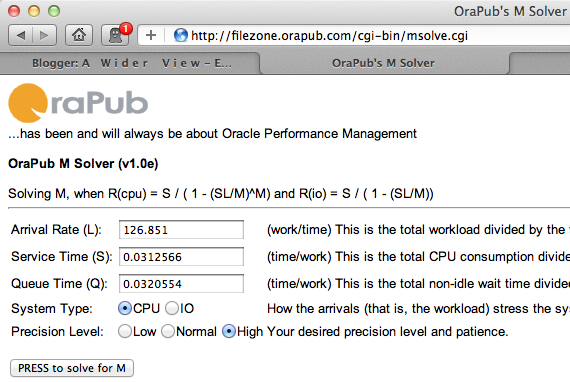
Figure 3.
Press the submit button to solve for M and in a few seconds you will receive what is shown in Figure 4.
Figure 4.
Figure 4 shows M at 4.598. There are four physical CPU cores in this system... not bad and very typical difference. (While I'm not going to go down this path, notice at the bottom of the Figure 4 there is a link to plot the resulting response time curve.) As Figure 4 shows, we now have all the variable values for the response time formula; M, L, S, Q, and R.Testing the Response Time Model
The question before us is, does the change in the service time (S) produce a corresponding change in the response time (R) as queuing theory states? Let's check!
Placing the modified service time (S) into our response time (R) formula along with the initial arrival rate (L) and effective servers (M):
R = S / ( 1 - ( L*S/M)^M )
= 0.0087205 / ( 1 - ( 126.851*0.0087205/4.59756)^4.59756 )
= 0.008733
Our model anticipates the response time to be 0.008733 ms/lio. The experimentally observed response time was 0.0093257 ms/lio. That's really close! As Figure 5 shows, the difference is only 6.4%.

Figure 5.
Figure 5 shows that when additional CBC latches were added and only incorporating the service time change into our response time model, the predicted response time differed only 6.4%. Considering the simplicity of our model, this is outstanding!You may have noticed that in Figure 1 when the additional latches where added and the system stabilized, the arrival rate increased by 175%. To be correct (and fair) to our response time model, we need to account for this change in the arrival rate. As most of you know, when we increase the arrival rate the resulting response time can also increase. So be fair, we need to incorporate the arrival rate increase into our model.

Figure 6.
Figure 6 shows the results when incorporating both the change in service time (S) and arrival rate (L) into the response time model. In this case, our prediction was off by 10%. Again, considering the simplicity of our model (which can be greatly enhanced as I discuss in my Oracle Forecasting & Predictive Analysis course), this is outstanding!Very cool, eh? What we have seen is that by tuning Oracle we have reduced the time it takes to process a logical IO (response time) and this reduction is as our classic CPU queuing theory based model indicates.
To Summarize...
The main point of this posting is to demonstrate that when we tuned Oracle by adding additional CBC latches, we effectively altered the Oracle kernel code path making it more efficient AND the resulting LIO response time changed as Operation Research queuing theory states!
In a little more detail, this is what occurred:
- There was an intense CPU bottleneck along with raging CBC latch contention.
- We observed the CPU time to process a single LIO (S) was 0.0313 ms and the total time to process a LIO (R) was 0.0633 ms.
- We increased the number of CBC latches from 256 to 32768.
- We restarted the system and let it stabilize.
- We observed the CPU time to process a single LIO (S) decreased by 72%, the arrival rate (L) increased by 175%, and the total time to process a LIO (R) decreased by 85%.
- Our response time model predicted, with the decrease in CPU time to process a LIO (S) and also the increase in the arrival rate (L), a response time (R) that was 10% greater than what actually occurred.
If this seems overly theoretical, in the next blog entry you'll see how we can use this information to anticipate the impact on a SQL statement's elapsed time!
Thanks for reading!
Craig.
If you enjoyed this blog entry, I suspect you'll get a lot out of my courses; Oracle Performance Firefighting and Advanced Oracle Performance Analysis. I teach these classes around the world multiple times each year. For the latest schedule, click here. I also offer on-site training and consulting services.
P.S. If you want me to respond with a comment or you have a question, please feel free to email me directly at craig@orapub .com. I use a challenge-response spam blocker, so you'll need to open the challenge email and click on the link or I will not receive your email. Another option is to send an email to OraPub's general email address, which is currently orapub.general@gmail .com.